Salsa al Parque - Solución

Salsa al Parque - Solución#

Tags: Parámetro binario, Variable Binaria, Scheduling

Enunciado#

El comité organizador del festival Salsa al Parque te ha contratado para definir el horario en el que se presentará cada uno de los cinco artistas principales. El comité le ha indicado que los artistas deben ser asignados a lo largo de una franja de 12 horas. En particular, hay un conjunto \(A\) de artistas y un conjunto \(H\) de horas. Salsa al Parque ha pronosticado la audiencia \(a_{it}\) que tendría cada uno de los artistas \(i\in A\) en caso de presentarse en cada hora \(t \in T\). Además, el comité estableció la duración \(d_{i}\) (horas) que debe tener la presentación de cada uno de estos artistas \(i\in A\). Para generar la planeación se definió la variable binaria \(x_{it}\) la cual toma el valor de uno si el artista \(i \in A\) inicia la presentación en la hora \(t \in H\) y cero de lo contrario. También, se decidió sobre la variable \(y_{it}\), la cual toma el valor de uno si el artista \(i \in A\) se presenta durante la hora \(t \in H\) y cero de lo contrario.

Debido a la importancia de cada uno de estos artistas, el comité enfatizó que todos los artistas se deben presentar una sola vez y que en cada hora se pueden presentar máximo dos artistas en simultaneo. Con el fin de propiciar presentaciones de calidad, el comité organizador te solicitó garantizar que cada artista realiza su presentación completa en horas consecutivas. El comité ha pedido definir las horas en las que se presentará cada artista de manera que se maximice la audiencia total. La Tabla 1 presenta la duración de la presentación y la audiencia esperada en cada hora para cada uno de los artistas.

Tabla 1. Audiencia esperada para cada artista en cada horario

		Audiencia (miles de personas)
		Hora
Artista	Duración Presentación (horas)	1	2	3	4	5	6	7	8	9	10	11	12
1	2	1197	2578	1350	2729	2679	2946	1563	2998	2879	1126	2559	1129
2	3	1034	2009	1515	2254	1624	1277	2010	2563	1384	2695	2053	2585
3	2	1058	1842	1443	1995	2819	1998	1401	1708	1346	1674	1816	1032
4	3	1082	1206	2366	1013	2762	1479	2496	1509	1673	1350	1128	2669
5	2	2801	1003	2965	2295	1147	2156	1058	2857	1968	2764	2153	1518

La siguiente tabla presenta una solución factible, aunque subóptima, para la situación planteada anteriormente:

Tabla 1. Configuración factible de los itinerarios.

	Hora
Artista	1	2	3	4	5	6	7	8	9	10	11	12
1		✓	✓
2					✓	✓	✓
3											✓	✓
4				✓	✓	✓
5										✓	✓

Formulación#

a. Formula matemáticamente un modelo de optimización de forma general que represente la situación anterior. Defina clara y rigurosamente:

Conjuntos
Parámetros
Variables de decisión
Restricciones
Naturaleza de las variables
Función objetivo

Conjuntos#

\(A\): artistas
\(H\): horas

Parámetros#

\(d_{i}\): duración de la presentación del artista \(i\in A\)
\(a_{it}\): audiencia del artista \(i\in A\) durante la hora \(t\in H\)

Variables de decisión#

\(x_{it}:\begin{cases}1\text{,}&\text{ si el artista }i\in A\text{ inicia su presentación en la hora }t\in H \\ 0\text{,}& \text{ d.l.c.} \end{cases}\)
\(y_{it}:\begin{cases}1\text{,}&\text{ si el artista }i\in A\text{ se presenta durante la hora }t\in H \\ 0\text{,}& \text{ d.l.c.} \end{cases}\)

Restricciones#

Se garantiza que la cantidad de artistas presentandose en simultaneo a cada hora \(h \in H\) sea menor o igual a \(k\):

\[ \sum_{i \in A}y_{i,t} \leq k,\ \forall t \in H; \]

Se garantiza que cada artista \(i \in A\) inicie su presentación una única vez:

\[ \sum_{t \in H}x_{i,t} = 1,\ \forall i \in A; \]

Se garantiza que cada artista \(i \in A\) se presenta en horas consecutivas y no presenta durante horas previas a la hora de inicio.

El artista \(i \in A\) se presenta en horas consecutivas desde el inicio de su presentación:

\[ \sum_{j = t}^{t+d_{i}-1}y_{i,j} \geq d_{i}x_{i,t},\ \forall i \in A, t \in H \ \vert\ t + d(i) - 1 \leq |H|; \]

El artista \(i \in A\) se presenta exactamente las horas que dura su presentación:

\[ \sum_{t \in H}y_{i,t} = d_{i},\ \forall i \in A; \]

El artista \(i \in A\) no puede iniciar su presentación si el tiempo restante es insuficiente:

\[ x_{i,t} = 0,\ \forall i \in A, t \in H \ \vert \ t + d_{i} - 1 > |H|; \]

Naturaleza de las Variables#

En cualquier instante \(t \in H\) un artista \(i\in A\) puede o no iniciar su presentación y puede o no estarse presentando.

\[ x_{it}, y_{it} \in \{0,1\},\ \forall i \in A, t \in H; \]

Función objetivo#

Se debe maximizar la audiencia total alcanzada.

\[ \operatorname{máx}\ \sum_{i \in A} \sum_{t \in H} a_{it}y_{it} \]

Implementación#

b. Resuelve el modelo planteado utilizando la librería de PuLP en Python. ¿Cuál es la solución óptima del problema?

Librerías#

Importa el módulo matplotlib.pyplot para crear gráficas y la librería pulp para crear y resolver el modelo.

import matplotlib.pyplot as plt
import pulp as lp

Conjuntos#

Define los conjuntos A y H que representan respectivamente los artistas y las horas.

Recuerda que por conveniencia de preservar el orden de los elementos de los conjuntos, no siempre deberás definirlos con el tipo set.

# Artistas
A = [f"A_{i}" for i in range(1, 6)]

# Horas
H = list(range(1, 13))

Parámetros#

Define o importa los parámetros del modelo.

# Duración de la presentación de cada artista
d = {"A_1": 2, "A_2": 3, "A_3": 2, "A_4": 3, "A_5": 2}

# Audiencia de cada artista en cada hora
a = {
    ("A_1", 1): 1197,
    ("A_1", 2): 2578,
    ("A_1", 3): 1350,
    ("A_1", 4): 2729,
    ("A_1", 5): 2679,
    ("A_1", 6): 2946,
    ("A_1", 7): 1563,
    ("A_1", 8): 2998,
    ("A_1", 9): 2879,
    ("A_1", 10): 1126,
    ("A_1", 11): 2559,
    ("A_1", 12): 1129,
    ("A_2", 1): 1034,
    ("A_2", 2): 2009,
    ("A_2", 3): 1515,
    ("A_2", 4): 2254,
    ("A_2", 5): 1624,
    ("A_2", 6): 1277,
    ("A_2", 7): 2010,
    ("A_2", 8): 2563,
    ("A_2", 9): 1384,
    ("A_2", 10): 2695,
    ("A_2", 11): 2053,
    ("A_2", 12): 2585,
    ("A_3", 1): 1058,
    ("A_3", 2): 1842,
    ("A_3", 3): 1443,
    ("A_3", 4): 1995,
    ("A_3", 5): 2819,
    ("A_3", 6): 1998,
    ("A_3", 7): 1401,
    ("A_3", 8): 1708,
    ("A_3", 9): 1346,
    ("A_3", 10): 1674,
    ("A_3", 11): 1816,
    ("A_3", 12): 1032,
    ("A_4", 1): 1082,
    ("A_4", 2): 1206,
    ("A_4", 3): 2366,
    ("A_4", 4): 1013,
    ("A_4", 5): 2762,
    ("A_4", 6): 1479,
    ("A_4", 7): 2496,
    ("A_4", 8): 1509,
    ("A_4", 9): 1673,
    ("A_4", 10): 1350,
    ("A_4", 11): 1128,
    ("A_4", 12): 2669,
    ("A_5", 1): 2801,
    ("A_5", 2): 1003,
    ("A_5", 3): 2965,
    ("A_5", 4): 2295,
    ("A_5", 5): 1147,
    ("A_5", 6): 2156,
    ("A_5", 7): 1058,
    ("A_5", 8): 2857,
    ("A_5", 9): 1968,
    ("A_5", 10): 2764,
    ("A_5", 11): 2153,
    ("A_5", 12): 1518,
}

# Máxima cantidad de artistas presentando en simultaneo
k = 2

Objeto del modelo#

Construye un problema al que luego agregarás las restricciones y la función objetivo.

problema = lp.LpProblem(name="scheduling-salsa-al-parque", sense=lp.LpMaximize)

Variables de decisión#

Define las variables del problema de manera que estén contenidas en diccionarios indexados en los conjuntos de sus variables respectivas.

# Si el artista a en A inicia su presentación en t en H
x = {
    (i, t): lp.LpVariable(
        name=f"inicia_{i}_en_hora_{t}", lowBound=0, upBound=None, cat=lp.LpBinary
    )
    for i in A
    for t in H
}

# Si el artista a en A se presenta durante la hora t in H
y = {
    (i, t): lp.LpVariable(
        name=f"presenta_{i}_en_hora_{t}", lowBound=0, upBound=None, cat=lp.LpBinary
    )
    for i in A
    for t in H
}

Función objetivo#

Agrega al problema la función objetivo. Recuerda que al definir el problema, ya definiste si este es de maximización o minimización.

problema += sum(a[i, t] * y[i, t] for i in A for t in H), "audiencia_total"

Restricciones#

Agrega al problema las restricciones del modelo.

# Los artistas presentandose durante h en H son menos que k
for t in H:
    problema += sum(y[(i, t)] for i in A) <= k

# Cada artista i en A inicia su presentación una única vez
for i in A:
    problema += sum(x[(i, t)] for t in H) == 1

# Cada artista se presenta en horas consecutivas luego de su inicio
for i in A:
    for t in H:
        if t + d[i] - 1 <= max(H):
            problema += sum(y[i, j] for j in range(t, t + d[i])) >= d[i] * x[i, t]

# cada artista debe presentarse exactamente la cantidad de horas que le corresponden
for i in A:
    problema += sum(y[i, t] for t in H) == d[i]

# Cada artista no puede iniciar su presentación si el tiempo es insuficiente
for i in A:
    for t in H:
        if t + d[i] - 1 > max(H):
            problema += x[i, t] == 0

Resolver el problema#

Invoca el optimizador. Este paso le asigna un valor a las variables incluidas en las restricciones o función objetivo del modelo.

problema.solve()

Welcome to the CBC MILP Solver 
Version: 2.10.8 
Build Date: May  6 2022 

command line - cbc /tmp/546f36a6114a4adeba154a11eba0f6e0-pulp.mps max timeMode elapsed branch printingOptions all solution /tmp/546f36a6114a4adeba154a11eba0f6e0-pulp.sol (default strategy 1)
At line 2 NAME          MODEL
At line 3 ROWS
At line 87 COLUMNS
At line 754 RHS
At line 837 BOUNDS
At line 958 ENDATA
Problem MODEL has 82 rows, 120 columns and 366 elements
Coin0008I MODEL read with 0 errors
Option for timeMode changed from cpu to elapsed
Continuous objective value is 32297 - 0.00 seconds
Cgl0002I 7 variables fixed
Cgl0003I 0 fixed, 0 tightened bounds, 53 strengthened rows, 0 substitutions
Cgl0003I 0 fixed, 0 tightened bounds, 47 strengthened rows, 0 substitutions
Cgl0003I 0 fixed, 0 tightened bounds, 16 strengthened rows, 0 substitutions
Cgl0003I 0 fixed, 0 tightened bounds, 12 strengthened rows, 0 substitutions
Cgl0004I processed model has 75 rows, 113 columns (113 integer (113 of which binary)) and 480 elements
Cbc0038I Initial state - 5 integers unsatisfied sum - 2
Cbc0038I Pass   1: suminf.    0.00000 (0) obj. -29428 iterations 38
Cbc0038I Solution found of -29428
Cbc0038I Before mini branch and bound, 107 integers at bound fixed and 0 continuous
Cbc0038I Full problem 75 rows 113 columns, reduced to 0 rows 0 columns
Cbc0038I Mini branch and bound did not improve solution (0.01 seconds)
Cbc0038I Round again with cutoff of -29525.5
Cbc0038I Reduced cost fixing fixed 18 variables on major pass 2
Cbc0038I Pass   2: suminf.    1.66667 (5) obj. -29904 iterations 8
Cbc0038I Pass   3: suminf.    1.66667 (5) obj. -29904 iterations 5
Cbc0038I Pass   4: suminf.    1.66667 (5) obj. -29904 iterations 4
Cbc0038I Pass   5: suminf.    2.14888 (10) obj. -29525.5 iterations 32
Cbc0038I Pass   6: suminf.    0.00000 (0) obj. -29681 iterations 19
Cbc0038I Solution found of -29681
Cbc0038I Before mini branch and bound, 92 integers at bound fixed and 0 continuous
Cbc0038I Full problem 75 rows 113 columns, reduced to 7 rows 5 columns
Cbc0038I Mini branch and bound improved solution from -29681 to -30024 (0.02 seconds)
Cbc0038I Round again with cutoff of -30099.7
Cbc0038I Reduced cost fixing fixed 42 variables on major pass 3
Cbc0038I Pass   7: suminf.    2.00000 (6) obj. -30155.8 iterations 1
Cbc0038I Pass   8: suminf.    1.66667 (5) obj. -30144.3 iterations 7
Cbc0038I Pass   9: suminf.    1.66667 (5) obj. -30144.3 iterations 2
Cbc0038I Pass  10: suminf.    1.90453 (9) obj. -30099.7 iterations 5
Cbc0038I Pass  11: suminf.    3.90354 (14) obj. -30099.7 iterations 33
Cbc0038I Pass  12: suminf.    2.00000 (8) obj. -30099.7 iterations 23
Cbc0038I Pass  13: suminf.    1.66667 (5) obj. -30099.7 iterations 5
Cbc0038I Pass  14: suminf.    2.17745 (9) obj. -30099.7 iterations 8
Cbc0038I Pass  15: suminf.    1.99482 (9) obj. -30099.7 iterations 11
Cbc0038I Pass  16: suminf.    2.00000 (8) obj. -30099.7 iterations 3
Cbc0038I Pass  17: suminf.    3.53805 (13) obj. -30099.7 iterations 14
Cbc0038I Pass  18: suminf.    2.00000 (8) obj. -30293.7 iterations 11
Cbc0038I Pass  19: suminf.    2.00000 (8) obj. -30293.7 iterations 1
Cbc0038I Pass  20: suminf.    2.22092 (9) obj. -30099.7 iterations 4
Cbc0038I Pass  21: suminf.    1.99482 (9) obj. -30099.7 iterations 1
Cbc0038I Pass  22: suminf.    2.00000 (8) obj. -30099.7 iterations 3
Cbc0038I Pass  23: suminf.    2.00000 (8) obj. -30099.7 iterations 4
Cbc0038I Pass  24: suminf.    1.66667 (5) obj. -30099.7 iterations 5
Cbc0038I Pass  25: suminf.    1.66667 (5) obj. -30144.3 iterations 3
Cbc0038I Pass  26: suminf.    1.90453 (9) obj. -30099.7 iterations 6
Cbc0038I Pass  27: suminf.    1.66667 (5) obj. -30144.3 iterations 16
Cbc0038I Pass  28: suminf.    4.00000 (11) obj. -30099.7 iterations 30
Cbc0038I Pass  29: suminf.    3.48328 (10) obj. -30099.7 iterations 8
Cbc0038I Pass  30: suminf.    3.48328 (10) obj. -30099.7 iterations 4
Cbc0038I Pass  31: suminf.    3.48328 (10) obj. -30099.7 iterations 3
Cbc0038I Pass  32: suminf.    2.00000 (6) obj. -30155.8 iterations 17
Cbc0038I Pass  33: suminf.    2.00000 (6) obj. -30155.8 iterations 9
Cbc0038I Pass  34: suminf.    1.66667 (5) obj. -30144.3 iterations 4
Cbc0038I Pass  35: suminf.    1.66667 (5) obj. -30144.3 iterations 3
Cbc0038I Pass  36: suminf.    1.90453 (9) obj. -30099.7 iterations 4
Cbc0038I No solution found this major pass
Cbc0038I Before mini branch and bound, 87 integers at bound fixed and 0 continuous
Cbc0038I Mini branch and bound did not improve solution (0.03 seconds)
Cbc0038I After 0.03 seconds - Feasibility pump exiting with objective of -30024 - took 0.02 seconds
Cbc0012I Integer solution of -30024 found by feasibility pump after 0 iterations and 0 nodes (0.03 seconds)
Cbc0038I Full problem 75 rows 113 columns, reduced to 0 rows 0 columns
Cbc0001I Search completed - best objective -30024, took 1 iterations and 0 nodes (0.03 seconds)
Cbc0035I Maximum depth 0, 38 variables fixed on reduced cost
Cuts at root node changed objective from -30402.5 to -28393.3
Probing was tried 0 times and created 0 cuts of which 0 were active after adding rounds of cuts (0.000 seconds)
Gomory was tried 0 times and created 0 cuts of which 0 were active after adding rounds of cuts (0.000 seconds)
Knapsack was tried 0 times and created 0 cuts of which 0 were active after adding rounds of cuts (0.000 seconds)
Clique was tried 0 times and created 0 cuts of which 0 were active after adding rounds of cuts (0.000 seconds)
MixedIntegerRounding2 was tried 0 times and created 0 cuts of which 0 were active after adding rounds of cuts (0.000 seconds)
FlowCover was tried 0 times and created 0 cuts of which 0 were active after adding rounds of cuts (0.000 seconds)
TwoMirCuts was tried 0 times and created 0 cuts of which 0 were active after adding rounds of cuts (0.000 seconds)
ZeroHalf was tried 0 times and created 0 cuts of which 0 were active after adding rounds of cuts (0.000 seconds)

Result - Optimal solution found

Objective value:                30024.00000000
Enumerated nodes:               0
Total iterations:               1
Time (CPU seconds):             0.04
Time (Wallclock seconds):       0.03

Option for printingOptions changed from normal to all
Total time (CPU seconds):       0.04   (Wallclock seconds):       0.04

Imprimir resultados#

Antes de estudiar el óptimo del modelo, identifica en el estado del optimizador si pudo resolver el problema.

f"Estado del optimizador: {lp.LpStatus[problema.status]}"

'Estado del optimizador: Optimal'

Identifica también el valor de la función objetivo.

f"Audiencia alcanzada: {lp.value(problema.objective) * 1000}"

'Audiencia alcanzada: 30024000.0'

Por último, imprime de manera estructurada el valor de las variables de decisión y otras expresiones de interés.

for t in H:
    print(f"\t{t}", end="")
print()

for i in A:
    print(i, end="")
    for t in H:
        print(f"\t{lp.value(y[i, t]): .0f}", end="")
    print()

	1	2	3	4	5	6	7	8	9	10	11	12
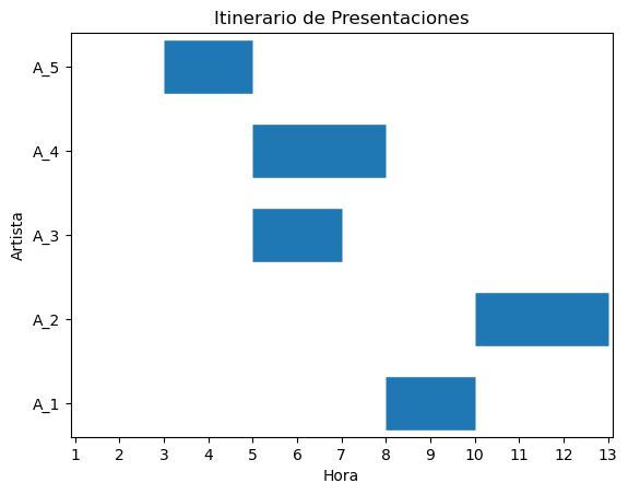
A_1	 0	 0	 0	 0	 0	 0	 0	 1	 1	 0	 0	 0
A_2	 0	 0	 0	 0	 0	 0	 0	 0	 0	 1	 1	 1
A_3	 0	 0	 0	 0	 1	 1	 0	 0	 0	 0	 0	 0
A_4	 0	 0	 0	 0	 1	 1	 1	 0	 0	 0	 0	 0
A_5	 0	 0	 1	 1	 0	 0	 0	 0	 0	 0	 0	 0

Visualizar resultados#

Ahora que conoces el valor de las variables de decisión, desarrolla una gráfica…

# Hora de inicio y hora de fin de cada artista.
comienzo = [sum(t * lp.value(x[i, t]) for t in H) for i in A]
fin = [comienzo[i] + d[f"A_{i + 1}"] for i in range(len(A))]

# Grafica de la solución
plt.hlines(A, comienzo, fin, linewidth=35)

# Etiqueta del eje x
plt.xlabel(xlabel="Hora")

# Etiqueta del eje y
plt.ylabel(ylabel="Artista")

# Título de la gráfica
plt.title("Itinerario de Presentaciones")

# Rango del eje x
plt.xlim([0.9, 13.1])

# Dígitos del eje x
plt.xticks(H + [13])

# Borde vacío al rededor de las barras
plt.margins(0.1)

../../_images/8a1689e22c82bae38c8e974676a77e2b60c83b86a63e9e2e061b9de7b60223e0.png

Créditos#

Equipo Principios de Optimización
Autores: Alejandro Mantilla, Ariadna De Ávila, Alfaima Solano
Desarrollo: Alejandro Mantilla, Alfaima Solano
Última fecha de modificación: 08/04/2023

Salsa al Parque - Solución

Contents

Salsa al Parque - Solución#

Enunciado#

Formulación#

Conjuntos#

Parámetros#

Variables de decisión#

Restricciones#

Naturaleza de las Variables#

Función objetivo#

Implementación#

Librerías#

Conjuntos#

Parámetros#

Objeto del modelo#

Variables de decisión#

Función objetivo#

Restricciones#

Resolver el problema#

Imprimir resultados#

Visualizar resultados#

Créditos#